FPGA Elementary Cellular Automata
A 1D cellular automata implemented on a Basys 3 board for CPE 133 final
February 2020 - March 2020
Source:
This is the report I submitted for the final project, transcribed into Markdown by hand, transformed into HTML by the static site generator, and rendered into pixels by your browser for your eyes to see.
Description
What is an elementary cellular automata?
An elementary cellular automata is a very simple model for computation. See this Wikipedia article for more information, or read my explanation here.
There is an array of cells that can have one of 2 states: either dead or alive. Every iteration, a rule is applied to every cell that looks somewhat like this:
| Current Pattern | 000 | 001 | 010 | 011 | 100 | 101 | 110 | 111 |
| New state for center cell | 1 | 0 | 0 | 1 | 0 | 0 | 0 | 1 |
where the current pattern is [left][center][right]. Assuming that the bordering cells are surrounded by 0, this is what will happen in one step of this rule:
| State 0 | 110011 |
| State 1 | 100010 |
Purpose of this project
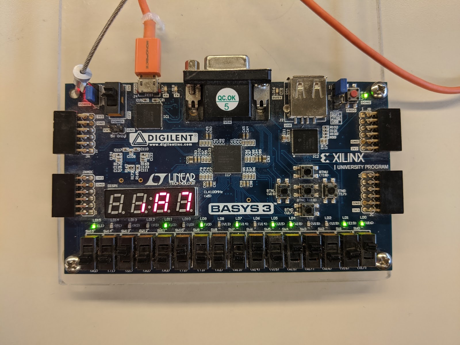
This project simulates a 1-dimensional cellular automata displayed on the LEDs. It provides an interface for the user to configure the initial state using the switches. Additionally, provides the user an interface to change the simulation rule and adjust the simulation rate through the 7-segment display.
Top-Level Black Box
![A schematic black box named top. Inputs: CLK, dec, dig_next, dig_prev, inc, reset, sw_IBUF[15:0], and toggle_BUFG. Outputs: an_OBUF[3:0], dp_OBUF, led_OBUF[15:0], seg_OBUF[6:0], and toggle_reg.](https://s3.us-west-000.backblazeb2.com/nyaabucket/0f2b461cbe0cea0d7b6082ab55a0ba1a18b004ce3dd1c6b1677fc3506b2d060b/blackbox.png)
Top-Level Structural Diagram
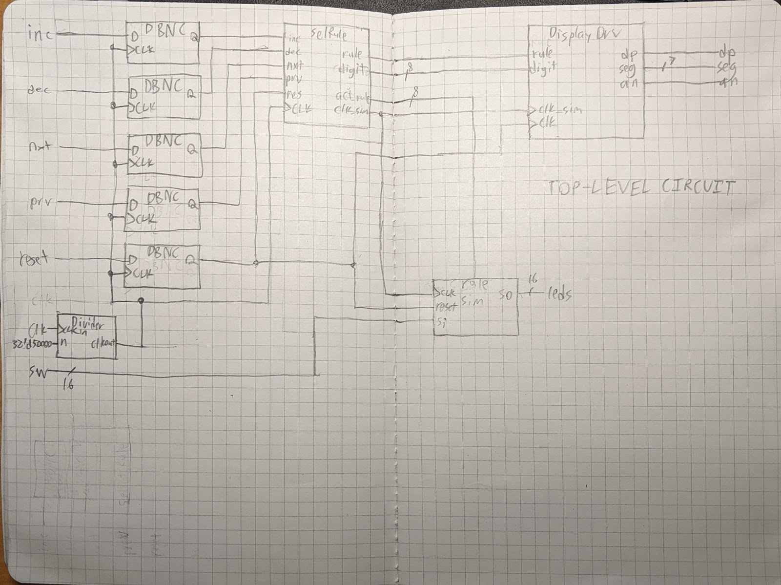
Notes
DBNCis the debouncing circuit found inDebouncer.svSelRuleis the submodule found inSelectRule.svDivideris the variable clock divider circuit found inClockDivider.svDisplayDrvis the submodule found inDisplayDriver.sv
Simulation Results
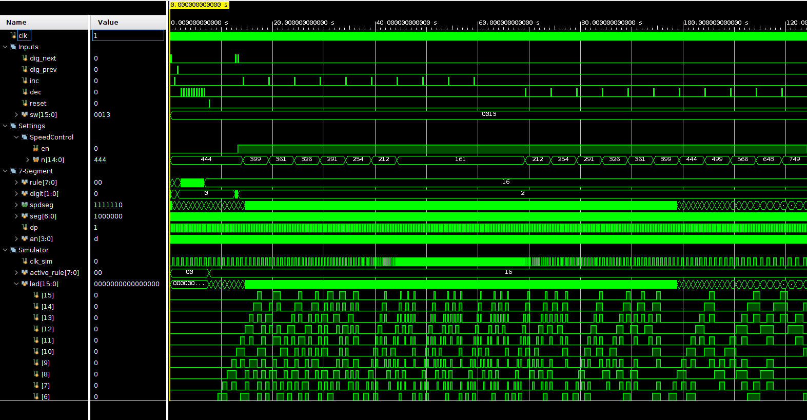
What this simulation does is:
- 0s to 10s: Set the rule to 16 by using
inc,dec, and the digit cursor.- Rule is changed, but
active_ruleis not changed untilResetis pressed.
- Rule is changed, but
- 12s to 60s: Increase the speed.
- The simulation clock accelerates during this time.
- The simulation clock divider
Ndecreases during this time.
- 65s to 120s: Decrease the speed.
- The simulation clock decelerates during this time.
- The simulation clock divider
Nincreased during this time.
Appendix A: Code
The code can be found on GitHub at https://github.com/ifd3f/Basys3-1D-Cellular-Automata.
Appendix B: Efficient, adder-only approximately constant-increment frequency selection
Motivation
I wanted to make it so that if you increment, you increase the frequency at a constant rate. Say we started at a clock divider output period of , or , and we wanted to increase the frequency by 0.1hz every time the increment button is pressed. We would have to change the period to , then , then , etc.
If I’m being completely honest, I didn’t need to do any of this, but I thought it would be cool at the time.
Implementation
Division is inefficient, so I decided to use an approximation to convert frequency to period. In the graph, the black curve is the function on , the bounds I want to restrict the simulator’s frequency to. The green curve is , which is the same function, but rescaled to and centered on the origin.
Approximation of
Let the third-order Taylor series approximation of be the cubic function . The blue function on the graph is the Taylor series approximation of it. I decided that the simulator would have 16 increments, so the actual function used is rescaled to centered at 8:
Optimization of
Since multiplication is slow and exponentiation is even slower, I decided to optimize the polynomial calculation using a third-order recursive sequence:
A third-order recursive sequence like this creates a sequence of numbers that lie on a cubic curve.
This allows us to calculate the result in a single clock cycle, and only using a few adders when going forward, or doing a small amount of subtraction when going backward.
I set and found the formulas for the initial values for these functions using a computer algebra system (specifically, a TI-92+):
The code that implements these formulas is in
SpeedControl.sv.